Exploring Argo Data Before You Write Code
OceanGraph helps you explore Argo float data before you start writing code.
When you begin oceanographic research, you are often told to “look at the data,” but it is not always clear what to look for or how to interpret what you see.
OceanGraph is a web-based visualization platform for searching Argo float profiles, inspecting trajectories and selected profile graphs, and viewing time-series vertical sections and θ–S diagrams. It helps you build intuition and develop research questions without dealing with NetCDF files or complex scripts.
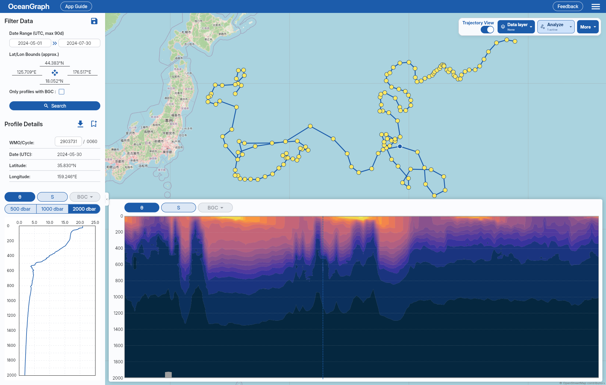
Open OceanGraph to explore real Argo profiles while reading this guide.
With OceanGraph, you can:
- View a selected profile graph and compare downloaded JSON profiles in Analysis Lab
- Examine water mass characteristics using θ–S diagrams
- Trace float trajectories to understand spatial context
- Identify patterns and anomalies that may lead to research questions
OceanGraph is not a replacement for numerical analysis or scripting. It is designed to support early-stage exploration and interpretation, not to produce final results for publication.
Start Exploring
Features
For everyone
- Search Argo floats worldwide by region and time (up to a 30-day date range)
- Search only profiles that include at least one BGC parameter
- Search by WMO ID for direct access to specific floats
- Track individual float trajectories
- Visualize time-series vertical sections of Argo float data
Note: Requests are rate-limited. Signing in does not increase an endpoint’s request limit.
For signed-in users
All free features, plus:
- Search Argo floats with an extended date range (up to 90 days)
- Visualize vertical profiles of temperature, salinity, oxygen, and supported BGC parameters
- View mixed layer depth from profile data
- View SOM (subsurface oxygen maximum) depth and its corresponding oxygen values
- Generate θ–S diagrams from up to 500 search-result profiles or up to 500 cycles in one trajectory
- Explore temperature, salinity, and six BGC variables down to 1000 dbar in a 3D view using up to 500 profiles in a selected region
- Download observation profile data for custom analysis
- Save screenshots of search results and visualizations
- Store up to 10 search bookmarks for repeated use
- Store up to 10 profile bookmarks for later reference or comparison
- Cluster up to 500 search-result profiles or up to 500 cycles in one trajectory
- Browse Ocean Basins and Mode Waters views in Visual Lab
- Upload and compare up to 30 custom JSON profiles in Vertical Profiles (desktop browsers only)
App Guide
This guide helps you start using OceanGraph, find the workflow that matches your goal, and understand the data behind the displays.
OceanGraph is a web application for searching and analyzing ocean observation data collected by the International Argo Program. You can search for temperature, salinity, dissolved oxygen, and other measurements from Argo floats based on geographic and temporal criteria, and explore the ocean state through various visualization and analysis features.
Open OceanGraph to follow this guide using the live application.
Start Here
Quick Start: Your First 10 Minutes
Follow one guided session from a map search to profile context, a float trajectory, a time-series vertical section, and an optional signed-in analysis.
Choose a Workflow
Usage Guide
Use the feature guides for one of OceanGraph’s three main workflows:
- Search and analyze profiles with Basic Features
- Browse precomputed regional views in Visual Lab
- Compare your own Argo-format JSON profiles in Analysis Lab
See Features for the current sign-in requirements and usage limits.
Understand the Data
Data Guide
Check the Argo data source, OceanGraph’s filtering policy, and limitations that affect how profiles, derived metrics, and missing areas should be interpreted.
Quick Start: Your First 10 Minutes
Follow this path from a map search to one float’s trajectory and an optional signed-in analysis.
Open OceanGraph and follow along.
Before You Start
You can complete steps 1–3 without an account. Profile graphs, analyses, and derived data layers require signing in.
See Features for the complete access and usage-limit reference.
Step 1: Search the map
- Set a Date Range (anonymous: up to 30 days; signed in: up to 90 days).
- Set the Geographic Bounds by interacting with the map.
- Optionally check Only profiles with BGC to keep profiles with biogeochemical measurements.
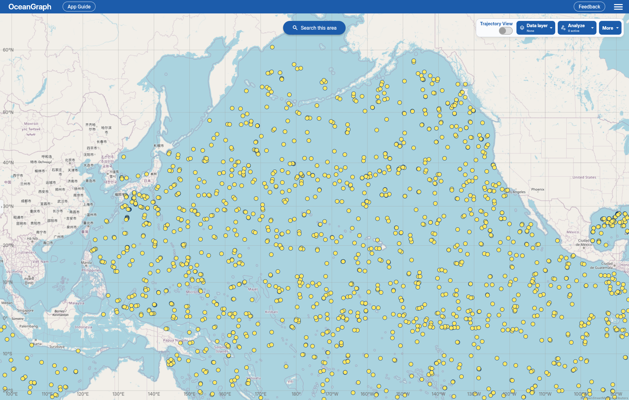
- Run the search. Matching profiles appear as markers on the map.
If you already know a float, enter its WMO ID in the Profile Details panel and press Enter to load all of its profiles.
See Search and Bookmark for details.
Step 2: Select a marker
Click a marker and read its profile context first: WMO ID, cycle number, date, latitude, and longitude. These details tell you which float, profile, place, and season you are about to interpret.
Signed-in users can also inspect the selected profile graph. Start with the overall shape of temperature or salinity and note the surface layer, the main gradient, and the deeper structure before moving to a multi-profile view.
Step 3: Follow One Float (Trajectory and Section)
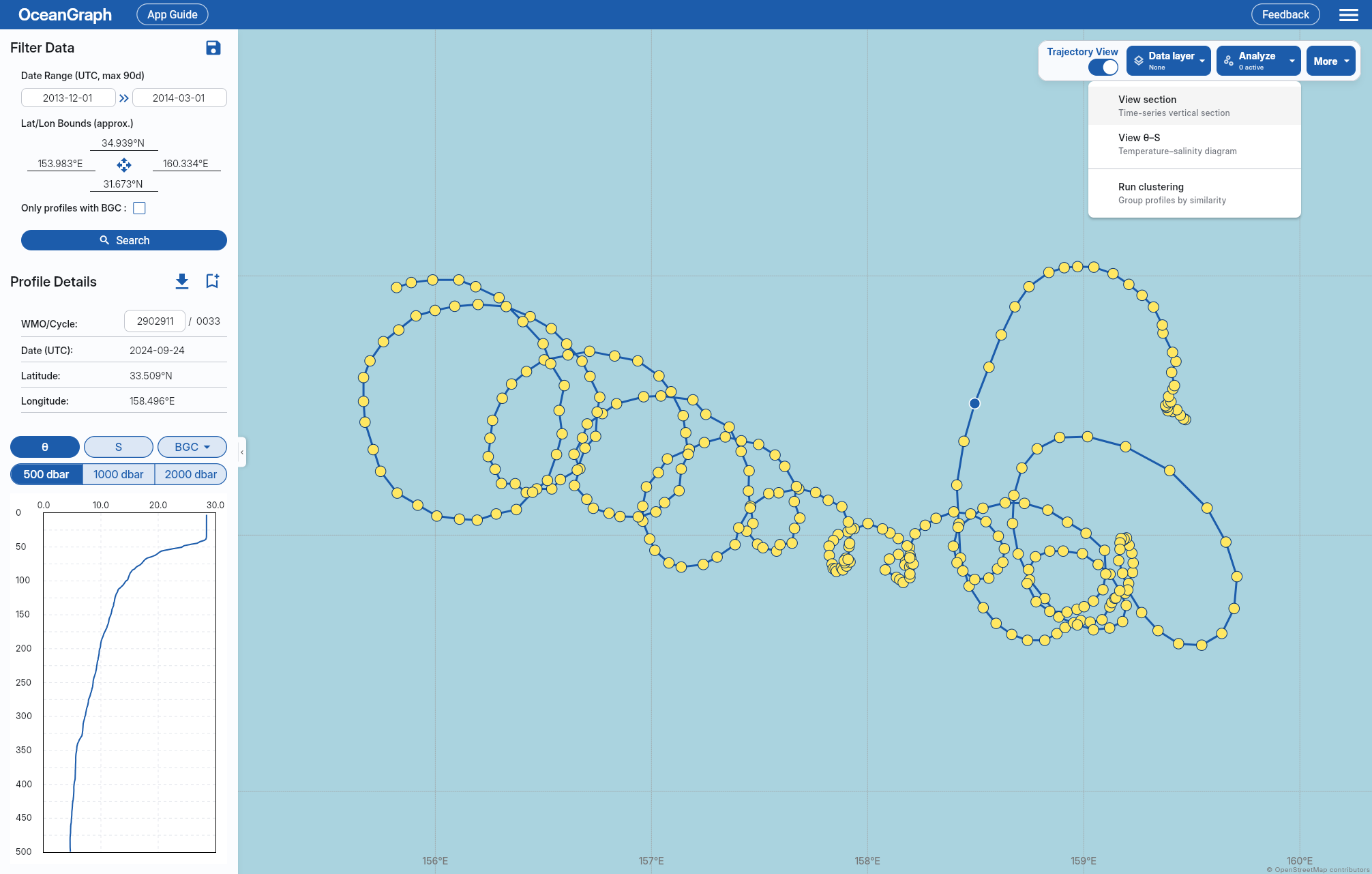
- In the map command bar, turn on Trajectory to load every cycle along the selected float’s trajectory.
- Open Analyze and select View section to see the time-series vertical section.
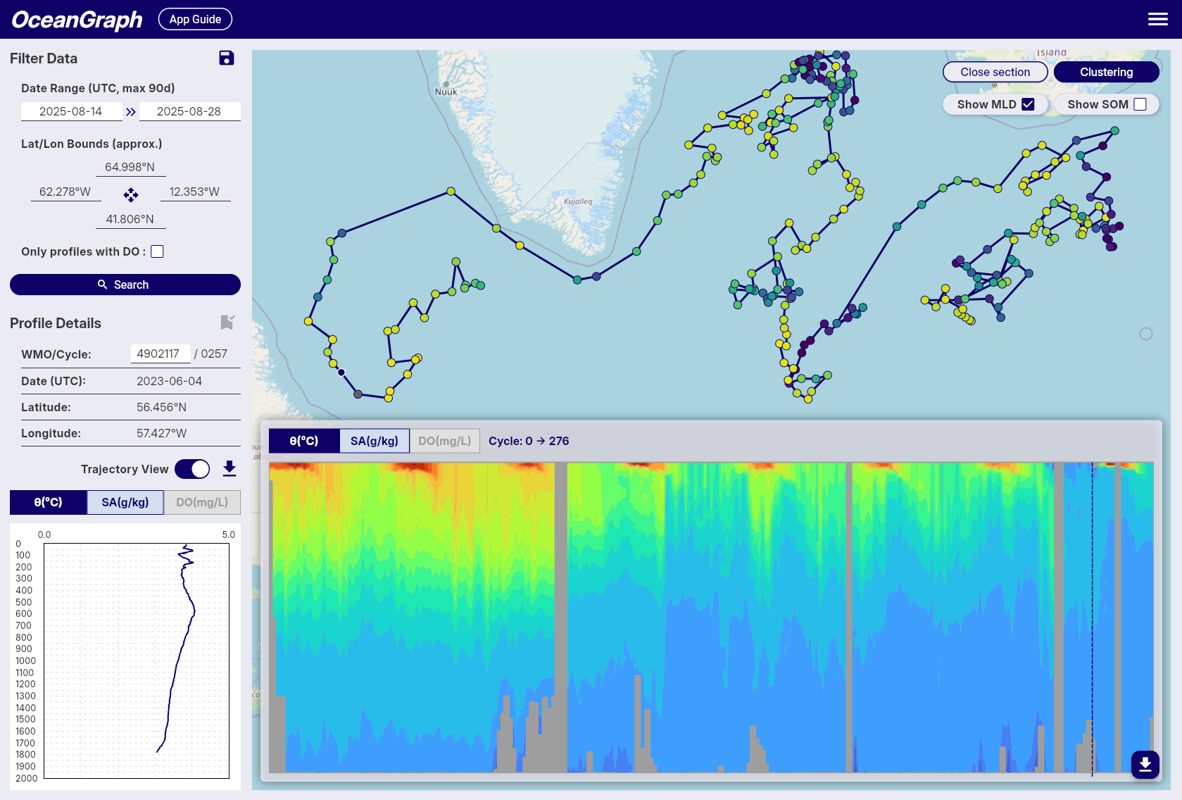
The dashed line marks the selected profile. Gray or blank areas indicate missing or insufficient data, not zero values.
See Trajectory and Time-Series Vertical Section.
Step 4: Choose an Analysis — Signed In
Open Analyze and select Generate θ–S to compare temperature-salinity structure, or Run clustering to group profiles by vertical structure. On narrower layouts, open Tools first.
With Trajectory off, these analyses use the current search results; with it on, they use all loaded cycles for the selected float. The limit is 500 profiles or cycles. Analyze shows progress, cancellation, and reasons for disabled actions.
See θ–S Diagram and Clustering.
Continue With Derived Data Layers
Signed-in users can choose one Data layer to color map markers:
- MLD: mixed layer depth; works with core Argo profiles.
- SOM: subsurface oxygen maximum; requires dissolved oxygen data from BGC profiles.
- Mode Water: detected layer thickness for a selected type, such as NPSTMW.
Gray or no-data markers indicate that a valid result is unavailable. MLD and SOM can also appear on the matching section chart.
If something doesn’t work
| Symptom | Likely cause and next step |
|---|---|
| No search results | The date range or area is too restrictive, or the BGC filter is on. Widen the range/area, or uncheck Only profiles with BGC. |
| θ–S or Clustering won’t run | The disabled item in Analyze gives the current count. With Trajectory off, narrow the date range or bounds to 500 profiles or fewer. With it on, a WMO with more than 500 cycles cannot be analyzed. |
| A feature is missing from the screen | θ–S, Clustering, MLD, SOM, mode water data layers, and downloads require signing in. Sign in and try again. |
| A chart is missing or has blank areas | Check Limitations for parameter availability, missing observations, and quality filtering. |
Where to go next
- Review the full Usage Guide and choose the workflow that matches your goal.
- Compare your own Argo-format JSON files in Vertical Profiles (signed-in, desktop only).
- Browse precomputed views in Visual Lab.
- Read the Articles for background on Argo floats, T-S diagrams, BGC parameters, and more.
Usage Guide
This section guides you through OceanGraph’s core functionality, from searching for Argo float data to visualizing and analyzing oceanographic observations.
Open OceanGraph to follow these workflows with real Argo data.
If this is your first session, begin with Quick Start: Your First 10 Minutes. For sign-in requirements and current limits, see Features.
OceanGraph provides three main workflows:
Basic Features
Search for profiles, inspect individual floats and trajectories, and open analysis views based on the current search results.
Visual Lab
Browse precomputed views of large-scale ocean patterns, including Ocean Basins and Mode Waters.
Analysis Lab
Work with your own Argo-format profile data. The current Vertical Profiles tool compares uploaded JSON profiles on desktop browsers.
Basic Features
These guides cover the search-based OceanGraph workflow, from finding profiles to opening visualizations and derived data layers.
Open OceanGraph to try these features in the live app.
For a guided first session, use Quick Start: Your First 10 Minutes. See Features for sign-in requirements and current limits.
- Search and Bookmark: find profiles by place, time, WMO ID, and BGC availability, then bookmark searches or profiles when signed in.
- Trajectory and Time-Series Vertical Section: follow one float and examine changes across its sequence of profiles.
- θ–S Diagram: compare potential temperature and absolute salinity relationships in search results or one trajectory.
- 3D View: select a region and compare horizontal temperature, salinity, and BGC distributions across pressure levels.
- Clustering: group search-result profiles or trajectory cycles by vertical structure for exploratory comparison.
- Mixed Layer Depth (MLD): color profiles by the automatically derived mixed layer depth.
- Subsurface Oxygen Maximum (SOM): inspect automatically detected subsurface oxygen maxima in BGC profiles.
- Mode Water Data Layer: compare profile-level mode water detections and layer thickness.
Search and Bookmark
OceanGraph provides search capabilities to find Argo float profiles based on geographic, temporal, and data quality criteria.
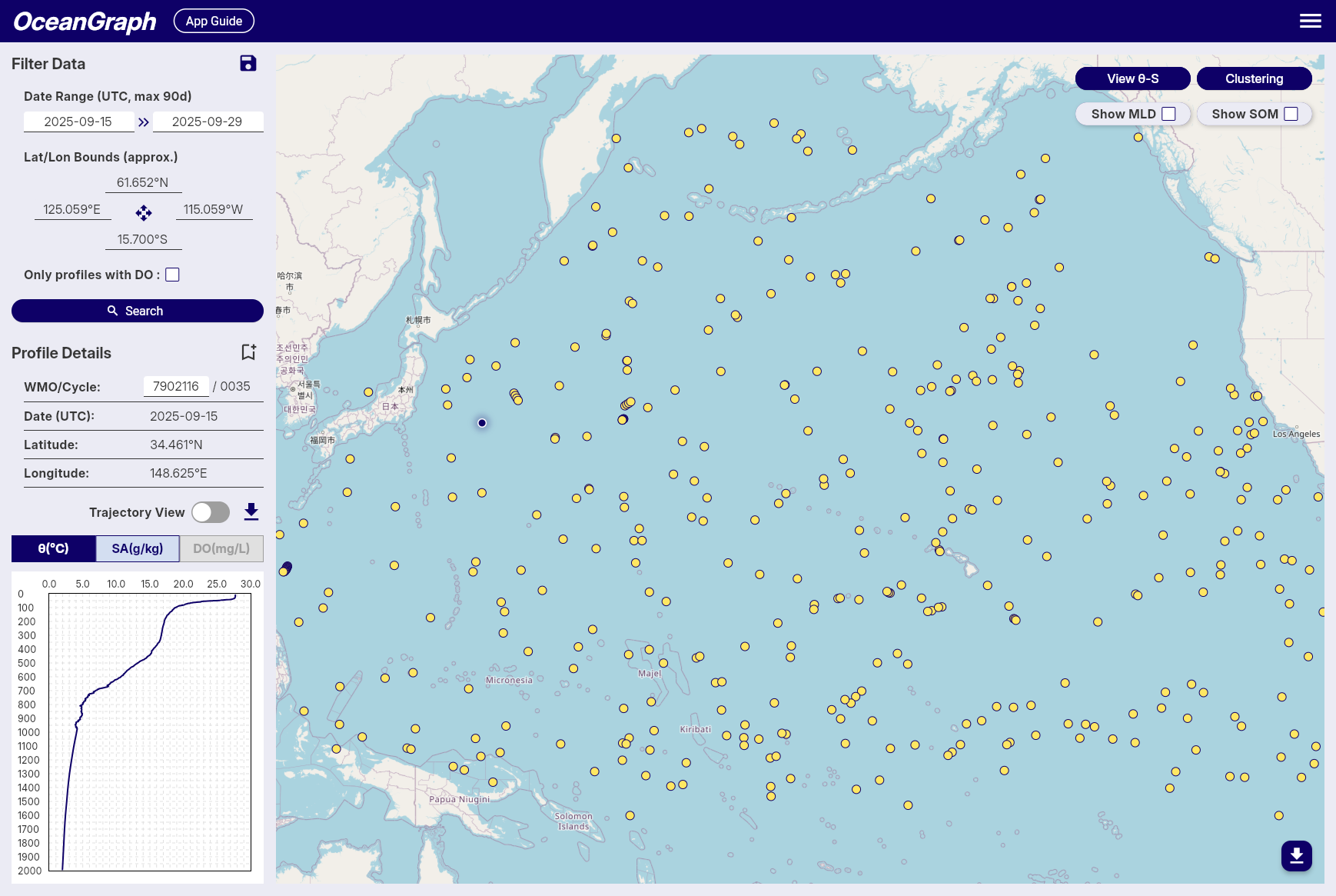
Search Methods
Control Panel
- Use the handle on the control panel’s right edge to hide or show it.
- The map command bar remains available while the panel is hidden. On narrower layouts, signed-in commands are grouped under Tools.
- After moving or zooming the map with the panel hidden, select Search this area to search the visible area with the current filters.
Filter Data Panel
-
Date Range
- Available: October 1999 to present
- Click date fields to select start and end dates
- All times in UTC
- Anonymous users can search up to a 30-day range; signed-in users can search up to a 90-day range
-
Geographic Bounds
- Move or zoom the map to set the search area
- With Trajectory off and the map focused, use the arrow keys to pan or + and − to zoom. See Trajectory navigation for selecting profiles with the arrow keys.
- Keyboard focus returns to the map on startup, after a successful search, and when returning from App Guide or Feedback. Mouse/touch selections in the controls also return focus to the map.
- Tab navigation, typing, menus, dialogs and chart controls keep keyboard priority. If you focus another control during a search, completion does not move focus back to the map.
- Select Lat/Lon Bounds (approx.) to view the coordinates
-
Data Availability
- “Only profiles with BGC” checkbox for profiles that include at least one supported BGC parameter: dissolved oxygen, chlorophyll, nitrate, backscattering, pH, downwelling irradiance at 490 nm, or PAR
- Not every BGC parameter has an in-app chart. Downwelling irradiance at 490 nm can be included in search and downloaded profile data, but it is not currently displayed as a chart.
-
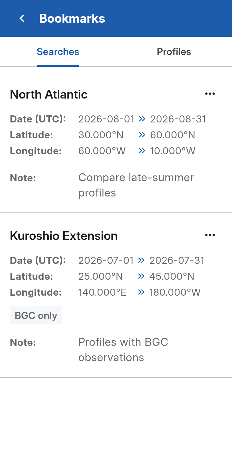
Bookmark Searches
Note: Available to signed-in users only
- Click Bookmark search (the bookmark icon) to create a search bookmark with the current search parameters
- Automatic naming by date range
- Up to 10 search bookmarks can be stored
Profile Details Panel
-
WMO ID Search
- Enter WMO ID and press Enter
- Returns all profiles for that specific float
-
Profile Information
- WMO ID, Cycle Number, Date (UTC), Latitude, Longitude
-
Bookmark Profiles
Note: Available to signed-in users only
- Click Bookmark profile (the bookmark icon) to create a profile bookmark
- A status indicator shows which profiles are already bookmarked, preventing duplicates
- Up to 10 profile bookmarks can be stored
-
Download Profile Data
Note: Available to signed-in users only
- Use Download profile beside the bookmark action in the Profile Details heading.
- The action becomes available only after the data for the currently selected WMO ID and cycle has loaded. It remains disabled while data is missing, loading, or belongs to an older selection.
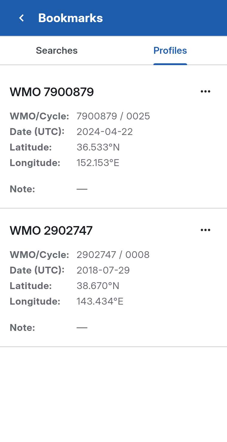
Using Bookmarks
Open Menu > Bookmarks, then choose the Searches or Profiles tab.
- Select a search card to search again with its saved filters, or a profile card to load its float and select the saved cycle when available. The drawer closes and keyboard focus returns to the map.
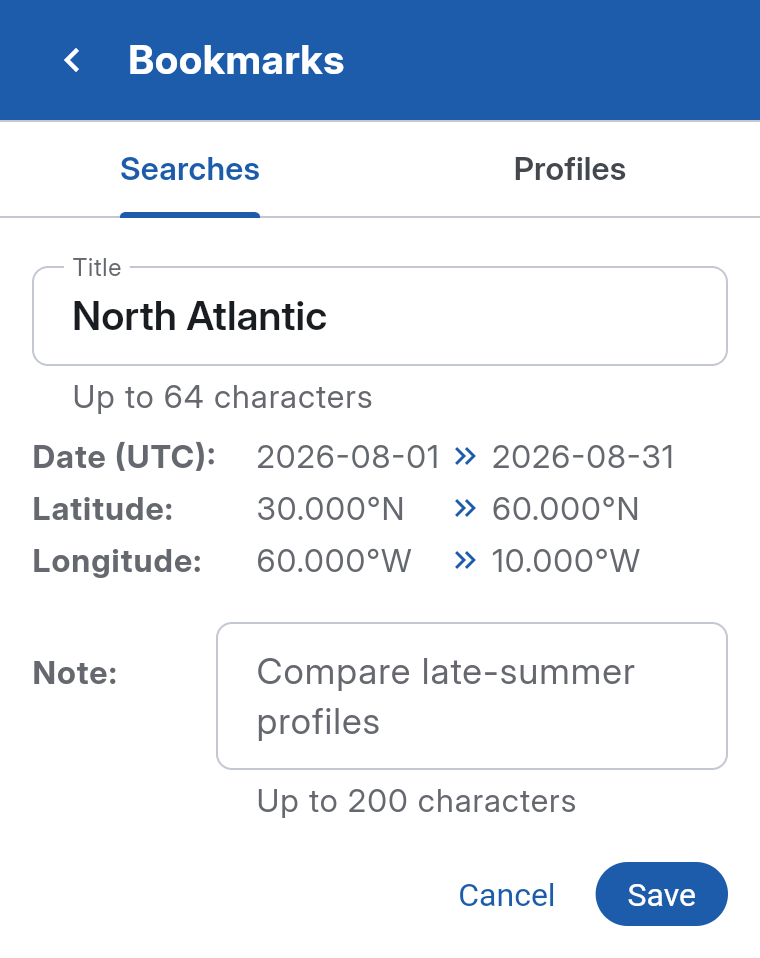
- Select ⋯ > Edit to change the title (up to 64 characters) or note (up to 200 characters), then select Save. Use Cancel to discard that item’s edits.
- Select ⋯ > Delete to remove a bookmark.
You can also focus a card with Tab and activate it with Enter or Space.
Save your edits before switching tabs, returning to the menu, or closing the drawer; otherwise they are discarded.
Results and Analysis Limits
Matching profiles appear as map markers; select one to open its details. If a search input is too broad for θ–S Diagram or Clustering, the corresponding Analyze item shows the current count and remains disabled. Narrow the date range or geographic bounds to 500 profiles or fewer. OceanGraph does not sample or split oversized inputs. Requests are also rate-limited; signing in does not increase an endpoint’s request limit.
For 3D View, the 500-profile limit applies to the selected rectangle, so a larger loaded set can still be narrowed on the map.
Related Reading
For guidance on choosing between regional, date-based, WMO ID, and BGC searches, read Finding Argo Float Profiles by Location, Time, and WMO ID in OceanGraph Articles.
Trajectory and Time-Series Vertical Section
Use a time-series vertical section to compare oceanographic parameters by pressure and profile cycle along one float’s trajectory.
Accessing Time-Series Vertical Sections
- Select a Float: Start by selecting an Argo float from the search results or the map view.
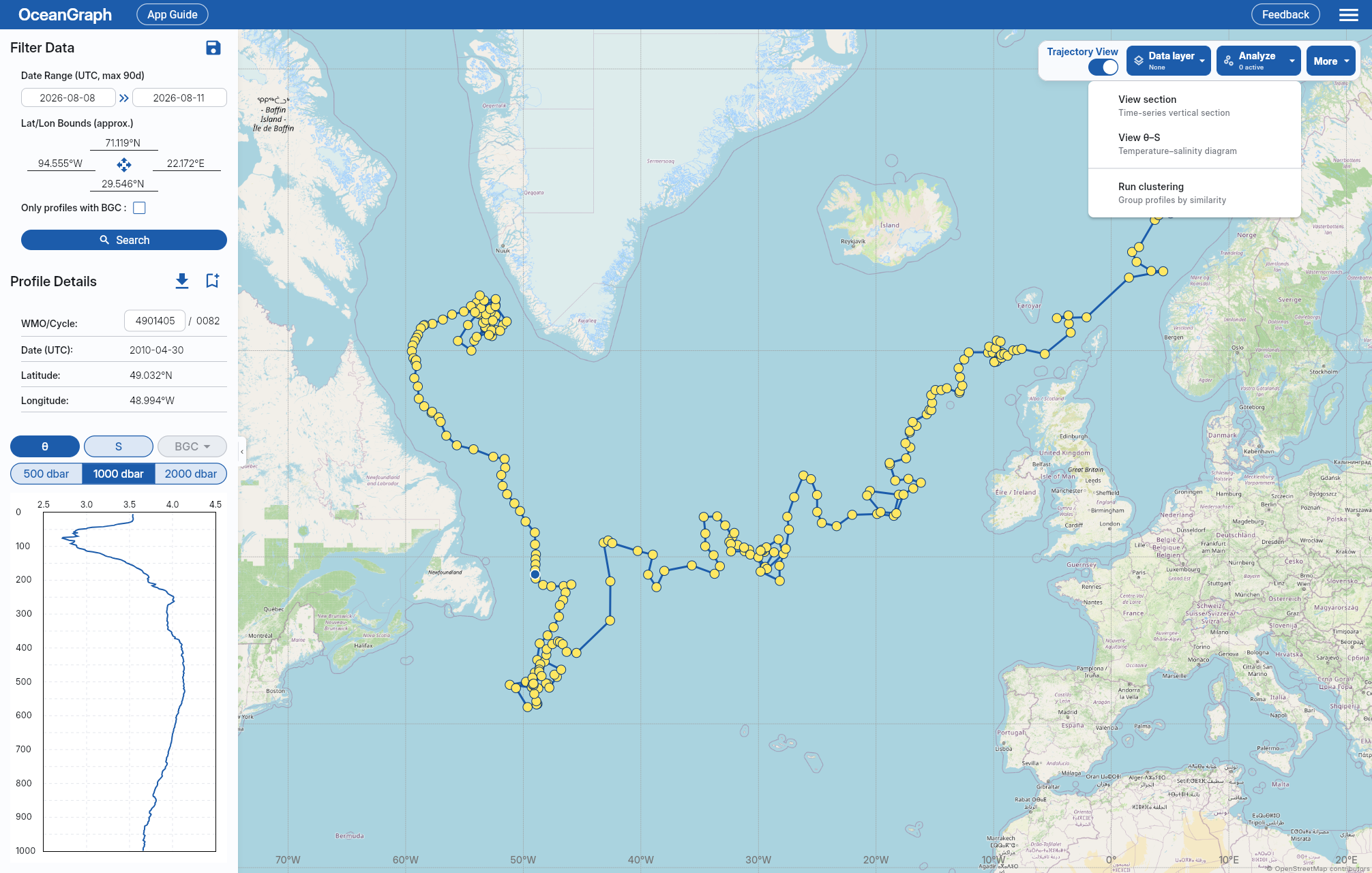
- Turn on Trajectory: In the upper-right map command bar, turn on Trajectory to load every cycle from the selected float’s trajectory. Trajectory is disabled until a profile is selected.
- Show vertical section: Open Analyze and select View section. On narrower layouts, open Tools, then use the same Analyze item.
- Choose a parameter: Use θ, S, or BGC above the section, independently of the Profile chart. Hover over, click, or tap BGC (or the selected variable name), then choose a variable.
During loading, the button immediately highlights and shows Loading… with a spinner; the map and selected profile remain visible. Once ready, it shows On with a checkmark. Click again or select another profile to cancel loading. If loading fails, it returns to Off with an error message; click again to retry.
The Date Range continues to show the filter used for the original search. Trajectory then loads all published cycles for the selected WMO ID, so Profile Details can show a cycle outside that range.
Turning Trajectory off restores the profile that was selected when it started, even if you moved to another cycle. Using the Trajectory button to turn it off also returns keyboard control to the map. A new search clears that saved selection. Toggling Trajectory closes the previous θ–S display, cancels an active θ–S or Clustering job, and closes the section when Trajectory ends.
With Trajectory on, ← / → select the previous or next profile, and none of the arrow keys pans the map. Mouse controls and map zoom shortcuts remain available. Text inputs, menus and the 3D view keep keyboard priority.
Signed-in users can also open θ–S from Analyze while Trajectory is on. θ–S and the section can be displayed together; θ–S uses every cycle in the selected WMO trajectory. When both charts are visible, selecting a profile updates the selected marker, the section’s dashed line, and the highlighted profile curve in θ–S together.
You can also generate a 3D view from loaded trajectory profiles within a rectangle. Toggling Trajectory cancels an unfinished 3D selection, but preserves generation already in progress and the latest successful result.
Interpret the Section
- The vertical section is linked with the vertical profiles in Profile Details, and the position of the selected profile is shown with a dashed line.
- Every parameter uses the same 0–2000 dbar coordinate at 5 dbar intervals. The 500 and 1000 dbar views crop this coordinate, so colors and MLD/SOM data-layer points remain aligned. Values are not extrapolated above the shallowest finite observation.
- Missing areas mean unavailable, masked, or insufficiently supported values, not zero. Interpolation is limited to pressure within a profile; missing cycles remain gaps.
- A parameter with a published section displays its chart. If individual profiles contain usable values but adjacent cycles do not provide enough support to draw a section, the parameter remains selectable and the section area explains the limitation. A parameter with no usable profile data is disabled.
- Signed-in users can show MLD or SOM with Data layer. Points mark valid results, and lines connect consecutive cycles only. Gaps indicate missing cycles or unavailable results; the lines are visual guides, not interpolation through time.
Related Reading
For help interpreting patterns, gaps, and changes across repeated profiles, read Time-Series Vertical Sections in Oceanography Explained in OceanGraph Articles.
θ–S Diagram
The θ–S diagram compares potential temperature and absolute salinity for either the current search results or one float’s loaded trajectory.
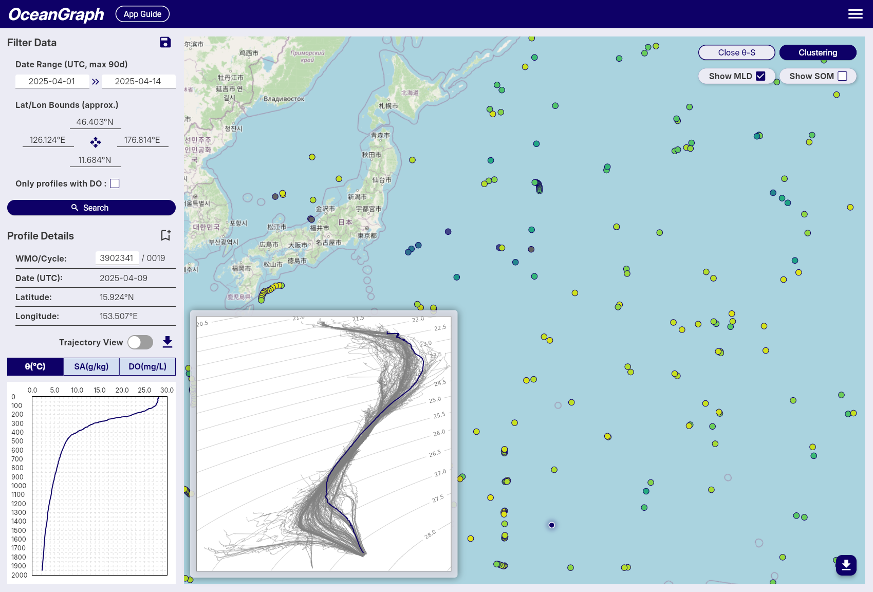
Open the Diagram
The diagram is available to signed-in users.
- With Trajectory off, run a search with no more than 500 profiles. With it on, select a WMO trajectory with no more than 500 cycles.
- Open Analyze in the map command bar and select Generate θ–S. On narrower layouts, open Tools first.
- Select a map marker to highlight that profile, or return to Analyze and select Close θ–S to hide the diagram.
The diagram uses the current search results with Trajectory off or every cycle in the selected WMO trajectory with it on. If a search exceeds 500 profiles, narrow the date range or geographic bounds. A trajectory over 500 cycles remains disabled; OceanGraph does not sample, split, or page either input.
While the diagram is being generated, Analyze shows progress and offers cancel or retry actions. The map remains usable. The latest result can be reopened without regeneration until you reset the search, leave Explore, or sign out.
With Trajectory on, θ–S and View section are independent and can remain visible together. When both are visible, selecting a map marker or using the left and right arrow keys changes the selected cycle in the marker, the section’s dashed line, and the highlighted θ–S profile curve together. Only one analysis job (θ–S, Clustering, or 3D view) can run at a time, but an already displayed θ–S diagram can still be closed while another job runs.
Read the Display
- The vertical axis is potential temperature and the horizontal axis is absolute salinity.
- Background contours show potential density anomaly referenced to 0 dbar (σ0). OceanGraph converts potential temperature to Conservative Temperature internally for this TEOS-10 density calculation; the plotted axes do not change.
- Each profile line uses pressure rows with a finite temperature-salinity pair. Profiles with fewer than two pairs are omitted.
- Unselected profiles use cluster colors, with excluded or unassigned profiles shown in gray. This is independent of the map’s Data layer.
- The selected profile appears in front as a thicker blue line.
Clustering and selection changes update the open diagram automatically.
Use the diagram to compare water-mass structure and mixing patterns. For a conceptual explanation, see T-S Diagrams in Oceanography Explained.
3D View
The 3D view stacks horizontal maps of potential temperature (θ), absolute salinity (S), and six BGC variables down to 1000 dbar. Use it to compare water properties across depths within a selected region.
Generate a View
Sign in and load profiles through a geographic search, a WMO ID search in Profile Details, or a profile bookmark. WMO searches and profile bookmarks use all loaded profiles for that float. With Trajectory on, the view uses its loaded cycles.
- Open Analyze, or Tools on a narrower screen, and select Generate 3D view.
- Drag on the map to draw a rectangle. The border snaps to a 0.5° grid and stops expanding at the size limit.
- Check the bounds and profile count in the bottom panel. Drag again to change the region, or select Cancel (Esc) to exit.
- Select Generate, or press Enter. The result opens when ready.
Select 1–500 profiles within the rectangle; only currently loaded profiles are used. The limit applies to the selected region, even if more than 500 profiles are loaded. The count updates while dragging; a red border indicates an empty or over-limit selection.
Changing the loaded data or toggling Trajectory cancels an unfinished selection. After Generate, the selected profiles and rectangle stay fixed.
After Generate, Cancel, or Esc, keyboard focus returns to the map, with normal or Trajectory navigation available during generation. When the result opens, keys operate the 3D view.
Progress and cancellation are available in Analyze / Tools. Only one analysis job can run at a time.
Read the View
Choose θ, S, or a variable from BGC: DOXY, CHLA, NO3, BBP, pH, or PAR. Variables with no valid values at any calculated pressure are disabled.
Open the depth menu beside the variable controls to choose Surface (10 dbar) or a level from 100 to 1000 dbar at 100 dbar intervals. The button shows the current depth, with Surface for 10 dbar; a check marks the selected menu item. Scroll within the menu to reach deeper levels. The selected layer is highlighted; other layers appear faintly in the background.
Dots show values derived from profiles at each pressure, and vertical lines connect the same profile. Thin rectangular frames mark the selected region at every pressure, including layers with no surface. Faint contours join equal values, while a latitude–longitude grid helps locate positions on the selected surface.
With Boost contrast off, each variable uses one color scale across all layers for comparing values across depths. Palettes match vertical sections, but their value ranges may differ.
Turn Boost contrast on to explore small differences within the selected layer. The same palette spans that layer’s minimum and maximum values, with a matching scale for its dots, surface, and contours. The legend shows physical values and units for that layer only, under Selected layer scale.
Faint background layers keep the normal shared scale, so the same color can mean different values on another layer or after changing depth. Even a small value range fills the palette; color differences do not establish scientific significance or identify anomalies. Contrast does not change values or fill missing areas.
Surface and profile values together set the contrast scale, including layers with only dots. A constant layer uses one color, no contours, and a legend showing only that value. A layer with no valid values has no color legend; follow its notice to find other data.
The header shows the total selected profiles; the count below the plot shows valid profiles for the current variable and pressure, matching the dots on that plane. Observation period covers all selected profiles, including those missing values for the current variable. It shows the earliest and latest UTC observation dates and stays the same when switching variables or pressure levels.
An information marker on a depth menu item or the selected depth button indicates insufficient data for a surface of the current variable. Open the menu and check the item’s tooltip for the reason. Levels and variables with only dots remain selectable. If no surface is available, try another variable, region, or set of profiles.
Surfaces show estimates only near valid observations for the selected variable and pressure. Areas farther away remain blank, including gaps between observation groups. See 3D view limitations for the distance limit, interpolation method, and accuracy limitations.
Navigate and Reopen
- Drag to rotate, or use the rotation buttons. Rotate up / Rotate down turn the view in the same direction as dragging upward / downward.
- Scroll or use Zoom in / Zoom out to zoom. Reset view restores the initial view without changing Boost contrast.
- Click or tap the Boost contrast switch beside the depth menu, or focus it with Tab and press Space. On a narrow screen, the switch moves to the next row.
- Use ↑ / ↓ for shallower / deeper levels and ← / → for the previous / next available variable, stopping at either end.
- Open the depth or BGC menu by hovering, clicking, or tapping its button. With the button focused, press ↓, Enter, or Space to open it. Hovering does not change the selection or keyboard focus.
- In an open menu, move focus with ↑ / ↓, then select with Enter or Space. Esc or a click outside closes it without selecting. The view behind the menu stays unchanged until selection; selecting or dismissing the menu returns keyboard focus to the view.
Changing depth, variables, or Boost contrast preserves the other selections, rotation, and zoom without recalculating the result. Each newly opened or reopened view starts with contrast off.
Select Reopen 3D view to return to the latest result without recalculation, or Generate 3D view to choose another region. Toggling Trajectory, or a failed or cancelled generation, keeps the latest successful result. Resetting the search, leaving Explore, or signing out clears it. Image and data export are not available from this view.
Clustering
OceanGraph provides an experimental feature that groups Argo profiles by similarities in their vertical structure and location.
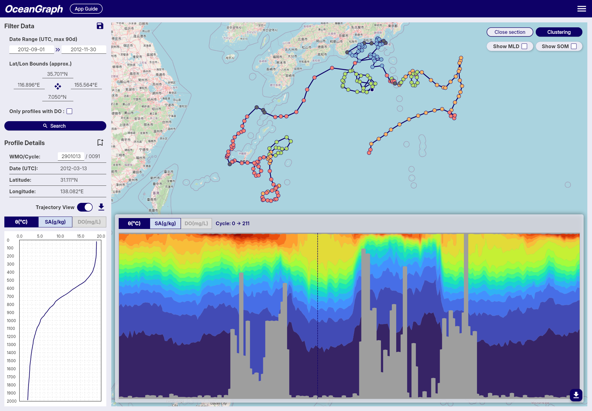
Accessing Clustering
Clustering is available to signed-in users only.
- Sign in. Leave Trajectory off to analyze the current search results, or turn it on to analyze the selected WMO trajectory.
- Keep the input at 500 items or fewer: current search-result profiles with Trajectory off, or all cycles for the selected WMO with it on.
- Open Analyze and select Run clustering. On narrower layouts, open Tools first.
- Follow the percentage on Analyze or Tools; the map markers are colored by cluster when processing finishes.
If the input exceeds the limit, the menu item shows the limit and current count and does not start a job. Narrow a Profiles search to recover availability. An oversized trajectory remains unavailable; OceanGraph does not sample, split, or page either input.
While Clustering runs, Analyze or Tools shows progress and provides cancel or retry actions. The map and existing displays remain usable. Only one analysis job (θ–S, Clustering, or 3D view) can run at a time.
Interpreting Results
- Colored markers indicate profiles assigned to clusters.
- Gray markers indicate profiles excluded from clustering because they did not satisfy the required variables or depth coverage.
- The cluster labels are exploratory groups, not confirmed water-mass names.
What the Grouping Uses
- Only pressure rows with a finite temperature-salinity pair are used.
- Profiles are compared on a shared 100 dbar grid from 200 dbar to an upper depth chosen from the input set, with 1000 dbar as the maximum. Profiles that do not cover that range are excluded.
- Temperature and salinity at each depth are standardized and combined with latitude and longitude.
- The number of clusters is selected automatically, up to six. A single eligible profile or identical inputs form one group.
Because the comparison depth and input population depend on the current selection, cluster numbers from different searches are not directly comparable.
Mixed Layer Depth (MLD)
OceanGraph derives a mixed layer depth exploration indicator from potential temperature, absolute salinity, and potential density anomaly referenced to 0 dbar (σ0).
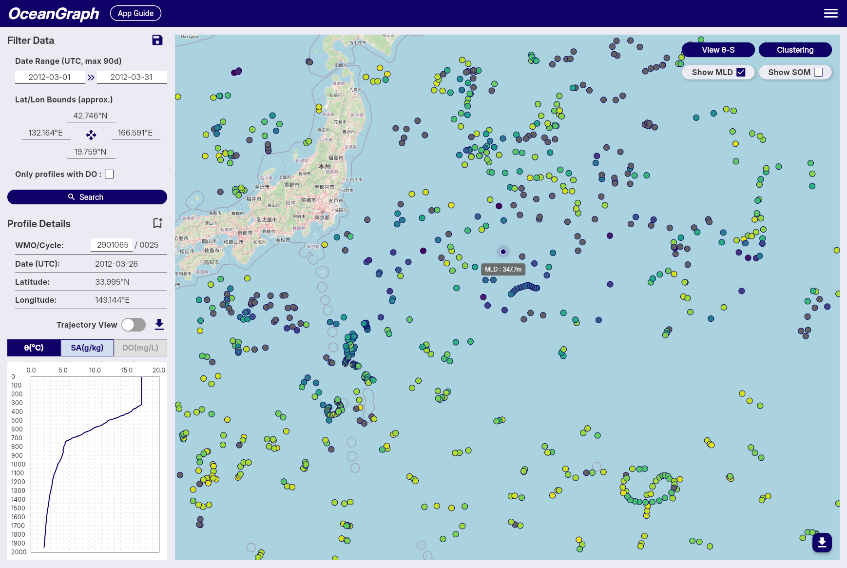
Use MLD
MLD is available to signed-in users.
- Search for profiles.
- Open Data layer in the map command bar and choose MLD. On narrower layouts, open Tools first.
- Compare marker colors and tooltip values.
- Select an observation to compare MLD with its vertical profile.
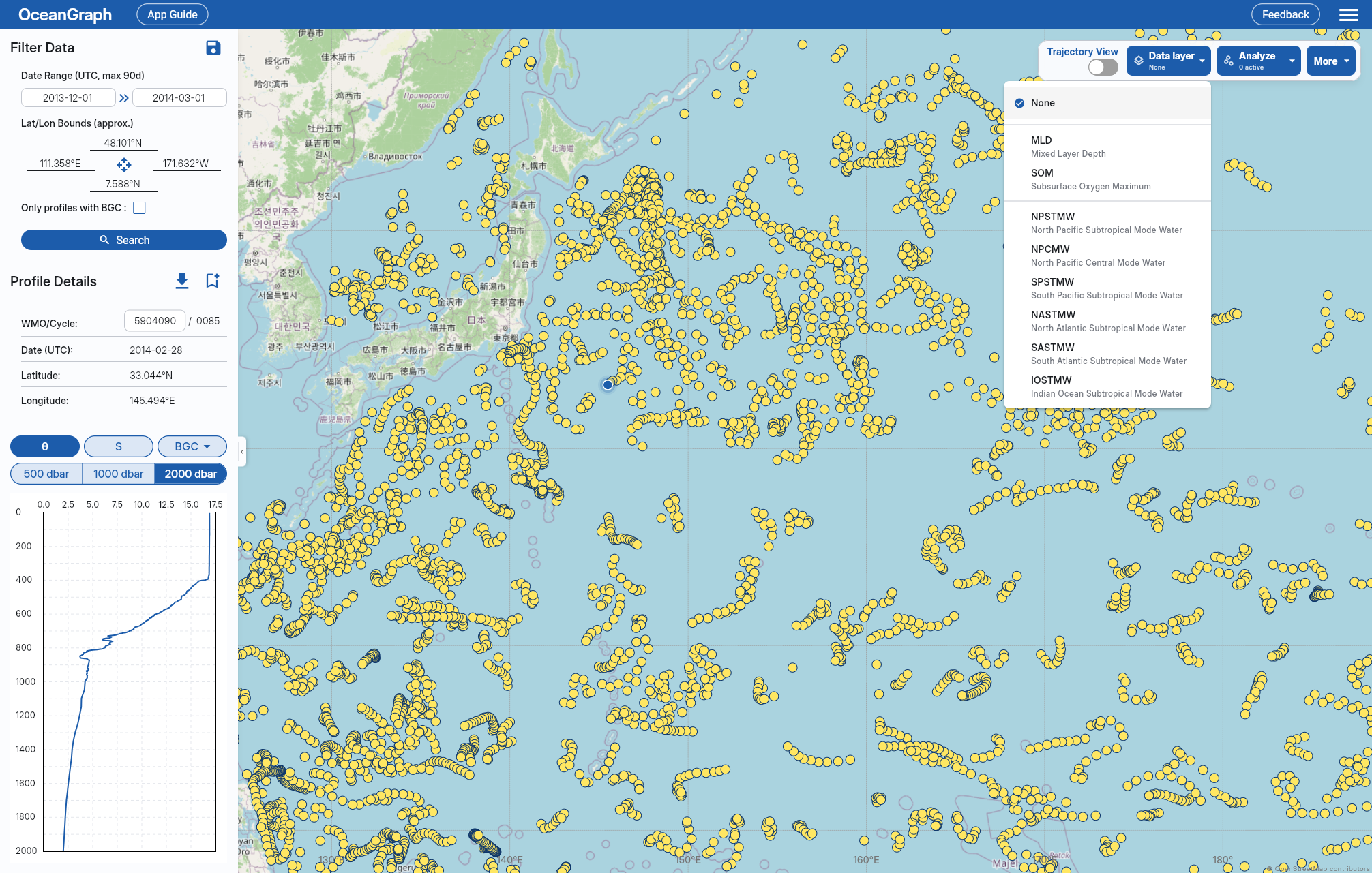
MLD, SOM, and mode water are mutually exclusive data layers. Profiles without a valid MLD are gray. Choose None to turn off the data layer.
The vertical profile shows MLD as a cyan dashed line when the selected observation’s curve is displayed and MLD falls within 0–Max (dbar). The line marks the same depth across displayed variables; Trajectory and a section are not required.
When Trajectory and a section are open, valid MLD values are shown as cyan points. Lines connect consecutive profile cycles only; they do not bridge missing cycles or imply interpolation through time.
Calculation
OceanGraph calculates three threshold crossings relative to the profile value at 10 dbar and uses the shallowest crossing.
| Criterion | Threshold |
|---|---|
| Potential temperature | 0.5 °C |
| Absolute salinity | 0.05 g/kg |
| σ0 | 0.125 kg/m³ |
Each crossing is linearly interpolated between the pressure rows that bracket its threshold and recorded to 0.01 dbar. Absolute salinity and potential temperature are derived with TEOS-10; Conservative Temperature is used only as an intermediate value for the density calculation.
The calculation requires at least three finite temperature-salinity rows, including two at 50 dbar or shallower. The shallowest paired row must be at 30 dbar or shallower and the profile must reach 10 dbar. If the first paired row is between 10 and 30 dbar, it supplies the reference values. If no threshold is crossed, MLD is undefined.
Map tooltips, vertical profiles, and section data layers use pressure in dbar. The color scale is a relative visual aid, and the result is an automatic threshold-based indicator rather than a guaranteed physical boundary. Because SOM selection begins below MLD, an MLD change can also change the reported SOM.
Subsurface Oxygen Maximum (SOM)
OceanGraph detects a supported local maximum in a profile’s dissolved oxygen measurements. SOM is an exploration indicator for upper-ocean oxygen structure, not a guarantee that every physical maximum will be detected.
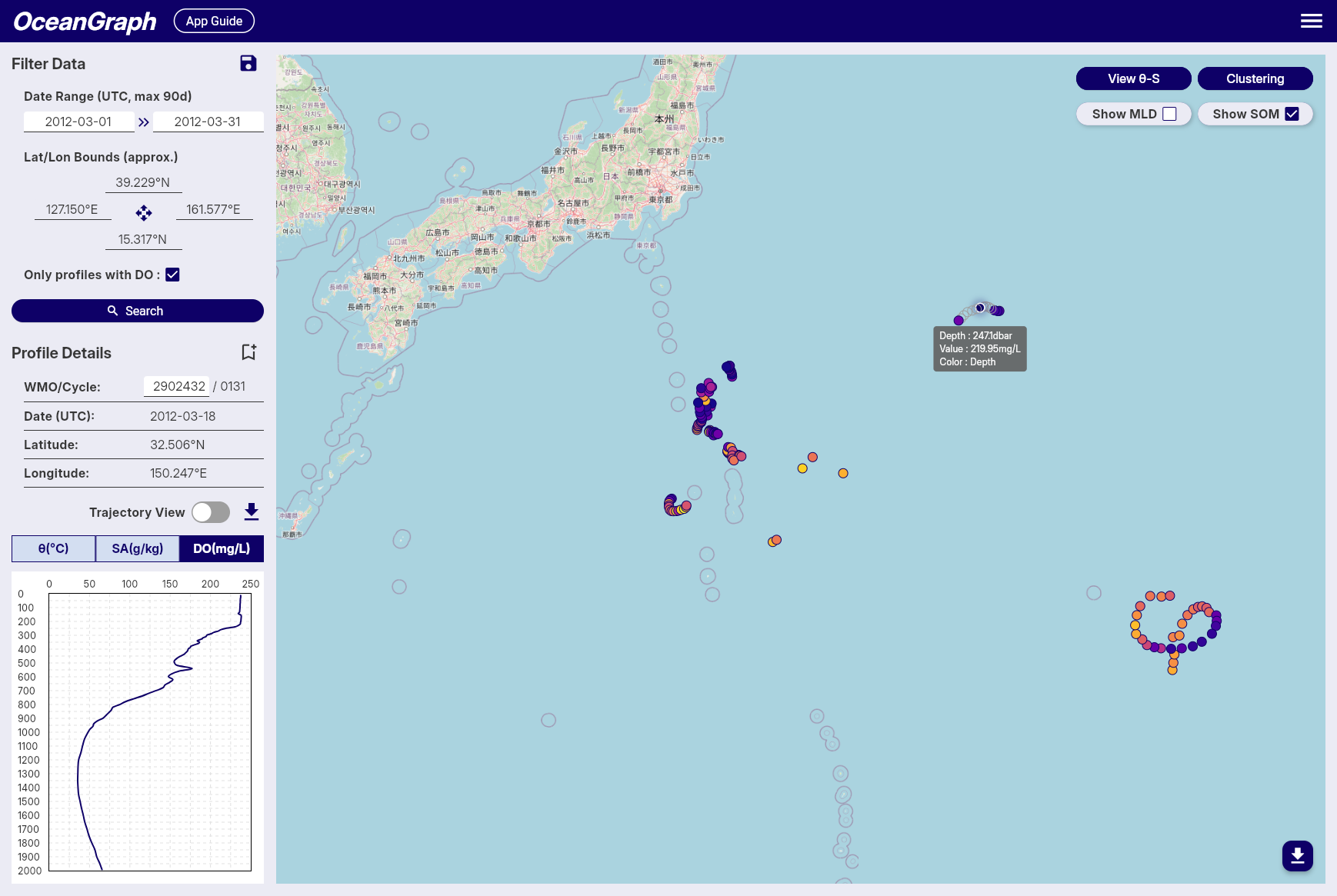
Use SOM
SOM is available to signed-in users and requires dissolved oxygen data.
- Search for profiles; use Only profiles with BGC to focus on BGC observations.
- Open Data layer in the map command bar and choose SOM. On narrower layouts, open Tools first.
- Compare SOM pressure and oxygen values in marker tooltips.
- Select an observation to compare SOM depth with its oxygen profile or another variable.
MLD, SOM, and mode water are mutually exclusive data layers. Profiles without oxygen or a valid SOM are shown as no-data markers. Choose None to turn off the data layer.
The vertical profile shows SOM as a purple dashed line when the selected observation’s curve is displayed and SOM falls within 0–Max (dbar). The line marks the same depth across displayed variables; Trajectory and a section are not required.
On an oxygen section, valid SOM values appear as purple points connected only across consecutive profile cycles. Gaps indicate a missing cycle or a profile where SOM was not detected or could not be calculated.
Detection
- With a valid MLD, candidates must be deeper than MLD and no deeper than 300 dbar. Without MLD, the range is 30–300 dbar. Profiles with MLD at 300 dbar or deeper are not assigned SOM.
- Detection uses finite source oxygen observations after quality masking and numeric-range checks. Internal gaps are interpolated only to evaluate peak shape; downloaded Profile JSON is not filled.
- A candidate must be an observed local maximum with at least 5 µmol/kg prominence and enough observed support around the peak. Endpoints, monotonic profiles, weak or unsupported narrow peaks, and peaks created only by interpolation are not reported.
- Candidates are ranked by prominence, oxygen value, then shallower pressure. When MLD exists, a supported peak within 100 dbar below MLD is preferred when available.
The result stores pressure in dbar and dissolved oxygen in µmol/kg. If no candidate satisfies the criteria, SOM is undefined.
Mode Water Data Layer
OceanGraph can color search-result map markers by profile-level mode water detection. This helps you inspect where individual profiles match a selected mode water type, and how thick the detected layer is.
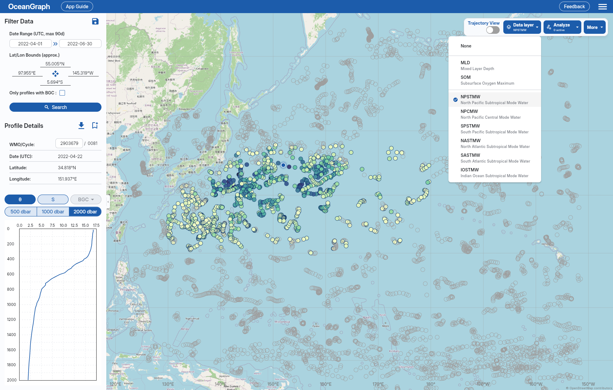
This data layer is separate from Visual Lab > Mode Waters. The data layer works on the profiles in your current search results, while Visual Lab shows precomputed three-month summaries and time series.
Accessing the Data Layer
The mode water data layer is available to signed-in users.
- Sign in and perform a search
- Open Data layer in the map command bar (or under Tools on a narrower layout)
- Choose one mode water type, such as NPSTMW or NASTMW
- Use marker colors and tooltips to compare detected layer thickness across profiles
Data layer is one exclusive menu containing None, MLD, SOM, and every supported mode water. Selecting a mode water replaces MLD or SOM coloring, and selecting MLD or SOM replaces mode water coloring. Choose None to return to the default marker colors.
Marker Colors and Tooltips
When a mode water type is selected:
- Profiles with that mode water are colored by detected layer thickness.
- Profiles without that selected mode water are shown as no-data markers.
- The tooltip shows the selected mode water type, layer thickness, core depth, and that marker color represents thickness.
Color represents thickness and should be read as a relative visual cue, not as a separate classification variable.
Supported Mode Water Types
The region column reflects OceanGraph’s default advection processing scope, which searches broader areas that can include advected mode water signals. Density ranges use potential density anomaly referenced to 0 dbar (σ0) in kg/m³.
| Short name | Full name | Region | Density range |
|---|---|---|---|
| NPSTMW | North Pacific Subtropical Mode Water | 20°N-38°N, 130°E-180° | σ0 = 25.0–25.6 kg/m³ |
| NPCMW | North Pacific Central Mode Water | 20°N-45°N, 145°E-145°W | σ0 = 26.0–26.6 kg/m³ |
| SPSTMW | South Pacific Subtropical Mode Water | 25°S-42°S, 150°E-170°W | σ0 = 25.8–26.5 kg/m³ |
| NASTMW | North Atlantic Subtropical Mode Water | 20°N-42°N, 85°W-35°W | σ0 = 26.3–26.6 kg/m³ |
| SASTMW | South Atlantic Subtropical Mode Water | 25°S-42°S, 60°W-20°E | σ0 = 26.2–26.7 kg/m³ |
| IOSTMW | Indian Ocean Subtropical Mode Water | 25°S-45°S, 20°E-70°E | σ0 = 25.8–26.2 kg/m³ |
All listed mode water types use a maximum potential vorticity threshold of 2 × 10⁻¹⁰ m⁻¹s⁻¹ and a minimum detected layer thickness of 10 m.
Detection Summary
OceanGraph checks quality-controlled, interpolated potential temperature and absolute salinity against the configured region, density, potential-vorticity, and minimum-thickness criteria. Where potential vorticity cannot be calculated, the density criterion is used alone. Core depth is the midpoint of the detected layer after converting its top and bottom pressures to depth; it is not the depth of minimum potential vorticity. A profile can contain more than one detected type, but the map displays only the type selected in Data layer.
Interpreting No-Data Markers
A no-data marker does not necessarily mean the profile is unusable. It means the selected mode water type was not detected for that profile under OceanGraph’s current automatic criteria. Common reasons include:
- The profile is outside the selected mode water’s geographic bounds
- The density or potential vorticity criteria were not met
- The matching layer was thinner than the 10 m minimum required thickness
- The profile did not have enough valid data after quality control and interpolation
Mode water detection is intended as an exploration aid. For research-grade classification, inspect the original profile structure and apply the criteria appropriate to your study.
Visual Lab
This section contains advanced visualization tools for analyzing large-scale oceanographic trends and water mass characteristics using Argo float data.
Visual Lab is available to signed-in users from Menu > Visual Lab in the live app.
Open OceanGraph to browse Visual Lab views in the live app.
Ocean Basins visualizes time series of average temperature and salinity changes across the world’s major ocean basins (North Pacific, South Pacific, North Atlantic, South Atlantic, and Indian Ocean) from 1998 to the present. This tool helps identify long-term oceanographic trends at regional scales.
Mode Waters detects and analyzes mode water layers in Argo float profiles based on density, potential vorticity, and thickness criteria. This feature provides time series visualization of mode water thickness trends and three-month distribution patterns.
Ocean Basins
Ocean Basins shows annual average potential temperature and absolute salinity at 10 dbar for the North Pacific, South Pacific, North Atlantic, South Atlantic, and Indian Ocean.
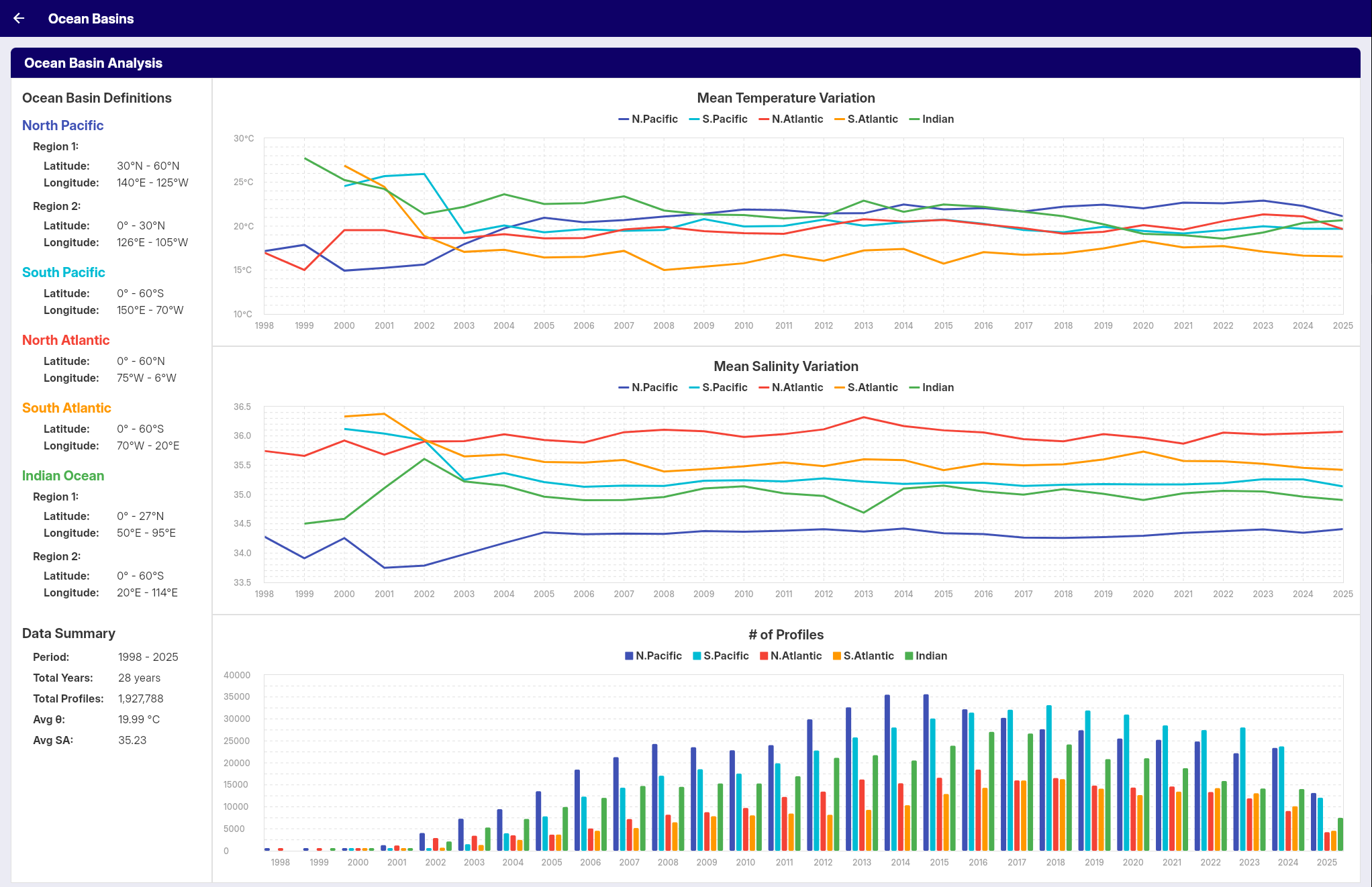
Accessing Ocean Basins
Sign in and open Menu > Visual Lab > Ocean Basins.
Read the Graphs
| Graph | Values |
|---|---|
| Temperature | Annual mean potential temperature (θ) at 10 dbar, by basin. |
| Salinity | Annual mean absolute salinity (SA) at 10 dbar, by basin. |
| Profile count | Number of Argo profiles used each year for each basin. |
The series runs from 1998 to the present and uses Argo profile measurements interpolated with the Akima method.
Interpretation Notes
- Early years have fewer Argo profiles than recent years, so check profile counts before comparing long-term values.
- The annual averages support exploratory visualization and education. Use original Argo data and a reproducible analysis workflow for publication-grade results.
Mode Waters
Mode Waters summarizes detected mode water layers by three-month period, with profile counts and thickness statistics.
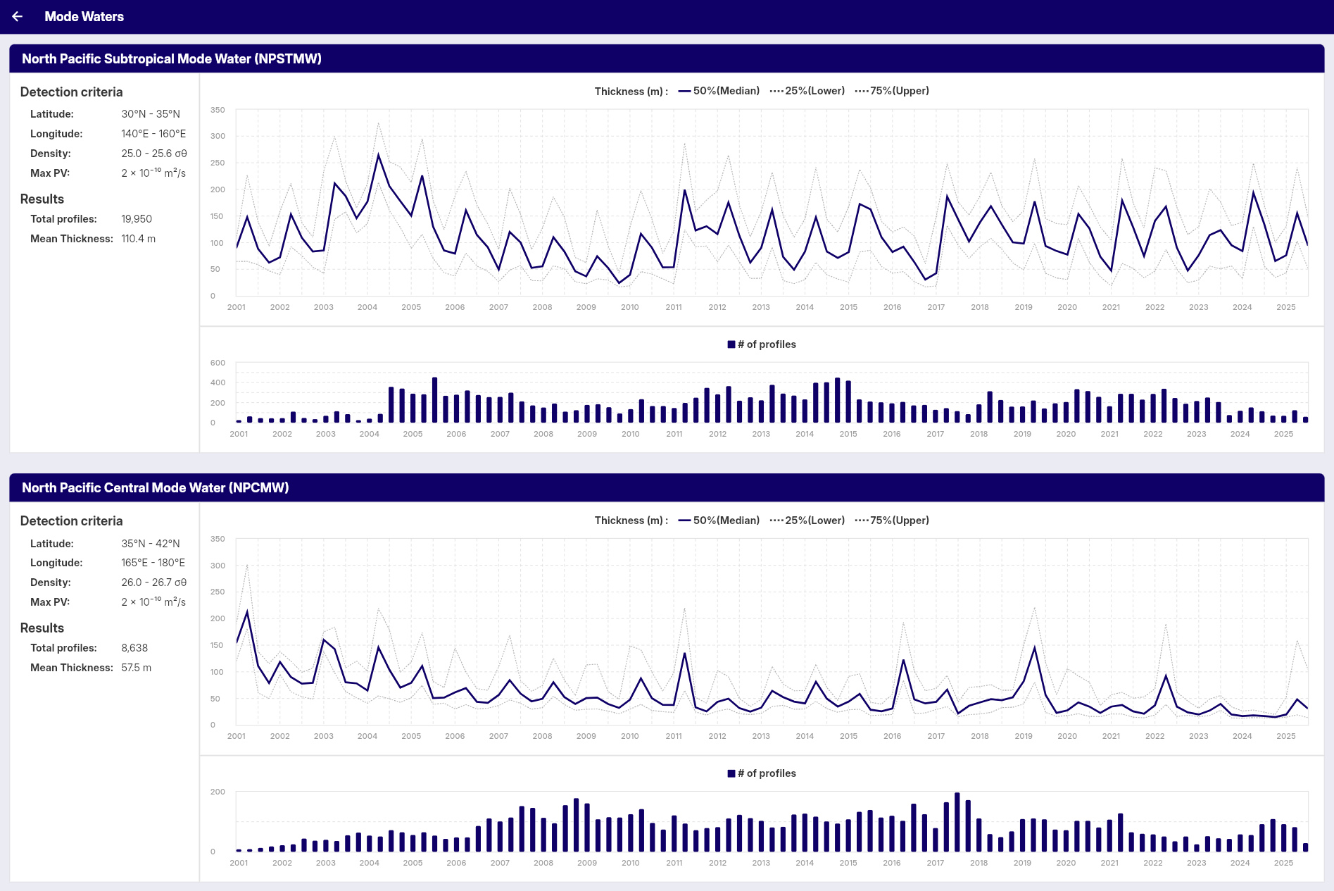
To inspect the same detections on individual map markers, use the Mode Water Data Layer.
Accessing Mode Waters
Mode Waters is available to signed-in users.
- Sign in to OceanGraph
- Open the app menu
- Select Visual Lab > Mode Waters
Results Display
The panel displays:
- Total Profiles: Number of profiles containing detected mode water layers
- Mean Thickness: Average of the three-month median thickness values shown in the time series
Graphs
Time Series Graph
Displays mode water thickness over time:
- Median Thickness: 50th percentile (solid blue line)
- Lower Quartile: 25th percentile (dashed gray line)
- Upper Quartile: 75th percentile (dashed gray line)
- Time Scale: Three-month periods from 2001 onwards
Profile Count Graph
Shows the number of profiles containing mode water:
- Blue Bars: Number of profiles per three-month period
- Time Scale: Three-month periods from 2001 onwards
Included Profiles
Detection uses the geographic bounds, density range, and potential vorticity threshold displayed on screen. Only profiles inside that region that reach at least 500 dbar and contain enough finite pressure, temperature, and salinity values are analyzed. Detected layers must be at least 10 m thick. Where potential vorticity cannot be calculated at a depth, the density criterion is used alone. These automatic criteria support exploration; they do not guarantee a research-grade water-mass classification.
Three-Month Periods
Data is grouped by month rather than by hemisphere-specific season names:
- DJF: December, January, February
- MAM: March, April, May
- JJA: June, July, August
- SON: September, October, November
Northern and Southern Hemisphere seasons are opposite, so a label such as DJF identifies only the months, not a local season. DJF uses the year of January and February: 2024 DJF covers December 2023 through February 2024. Graph tooltips show only the concrete month range, such as Dec 2023–Feb 2024 or Mar–May 2024.
Related Reading
For background on mode-water formation and interpretation, read What Is Mode Water? in OceanGraph Articles.
Analysis Lab
Analysis Lab is available to signed-in users from Menu > Analysis Lab in OceanGraph.
The desktop-only Vertical Profiles tool compares uploaded Argo-format JSON profiles and exports charts with an optional note.
Vertical Profiles
The Vertical Profile Viewer is a feature of OceanGraph that allows you to visualize and compare vertical profiles of oceanographic data.
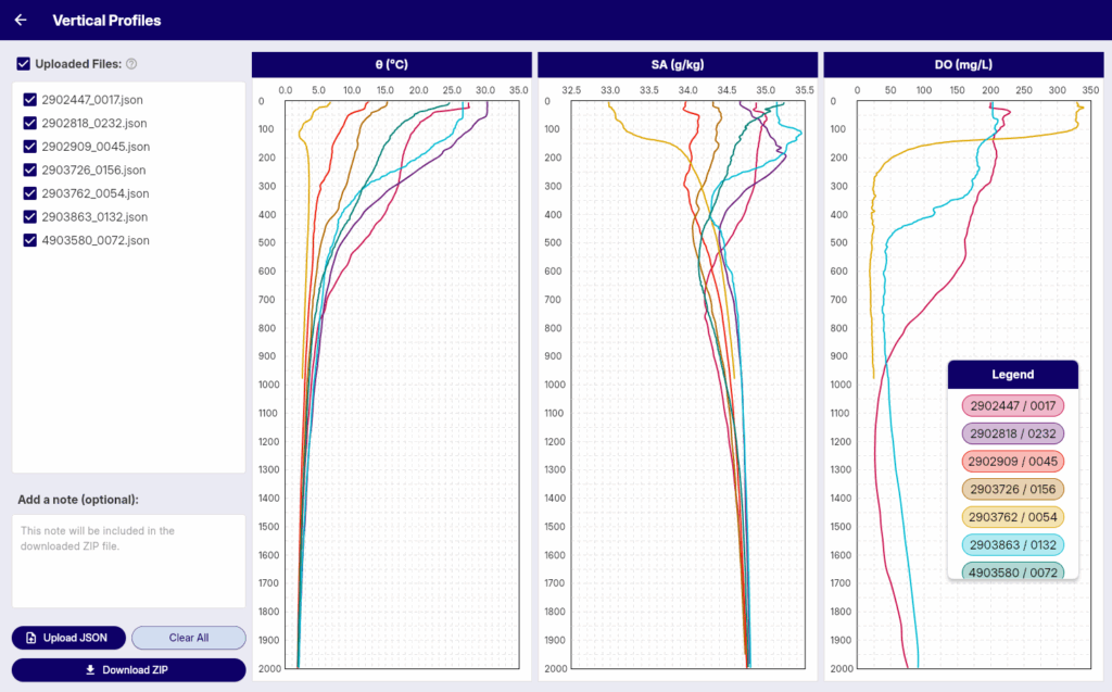
With this tool, you can:
- Upload one or more JSON files containing vertical profile data.
- Visualize temperature, salinity, dissolved oxygen, and supported optional BGC variables by depth;
nullstays missing, and charts connect two or more finite cells with straight lines. - Add a brief note that is included in the downloaded ZIP file.
- Download profile charts and the note as a ZIP file.
Access and Limits
Vertical Profiles is available to signed-in users on desktop browsers only.
- Open Menu > Analysis Lab > Vertical Profiles in the live app.
- Upload up to 30 JSON files.
- If you upload a file with the same filename as an existing uploaded file, the previous file is replaced.
- Select or deselect uploaded files to control which profiles are shown in the charts.
- Use Clear All to remove uploaded files and clear the note.
The downloaded ZIP contains one PNG file for each chart type and note.txt. The draggable legend is available in the viewer only.
Supported JSON Format
Each JSON file must contain the following keys:
{
  "pressure": [ ... ],
  "potential_temperature": [ ... ],
  "absolute_salinity": [ ... ],
  "oxygen": [ ... ],
  "wmo_id": "2902447",
  "cycle_number": 17
}
"pressure": array of numbers (required, must not be empty)"potential_temperature": array of numbers or nulls (required; if non-empty, same length aspressure)"absolute_salinity": array of numbers or nulls (required; if non-empty, same length aspressure)"oxygen": array of numbers or nulls — dissolved oxygen concentration (μmol/kg) (required; if non-empty, same length aspressure)"wmo_id": string or number (required, up to 20 characters after conversion to text)"cycle_number": number (required)
Optional BGC keys can also be included:
"chlorophyll": array of numbers or nulls — chlorophyll-a (mg/m³) (same length aspressure, if present)"nitrate": array of numbers or nulls — nitrate (μmol/kg) (same length aspressure, if present)"bbp700": array of numbers or nulls — particulate backscattering at 700 nm (m⁻¹) (same length aspressure, if present)"ph": array of numbers or nulls — in-situ pH (same length aspressure, if present)"irradiance490": array of numbers or nulls — downwelling irradiance at 490 nm (W/m²/nm) (same length aspressure, if present). This key is accepted, but it is not displayed as a chart in the current interface."par": array of numbers or nulls — photosynthetically available radiation (μmol/m²/s) (same length aspressure, if present)
Any additional keys will be ignored. Files that do not follow the required structure or fail validation will be skipped during upload.
Related Reading
For a beginner-friendly explanation of profile context, variables, quality information, and vertical structure, read How to Read Argo Float Data for Beginners in OceanGraph Articles.
Data Guide
This section explains where OceanGraph data comes from, how profiles are filtered, and what limitations to keep in mind when interpreting results.
Open OceanGraph to inspect the live dataset while reading this guide.
OceanGraph aims to refresh its data weekly. Update notices and current availability are posted on X (Twitter) at @OceanGraphJP.
Data Source
OceanGraph uses Argo float data and associated metadata provided by the International Argo Program and the national programs that contribute to it. These data are made freely available through the Argo Global Data Assembly Centre (Argo GDAC) and are a core component of the Global Ocean Observing System (GOOS).
For data access, OceanGraph retrieves Argo GDAC files via the public AWS S3 distribution (Open Data on AWS), which is synchronized with the GDAC holdings and updated on a daily basis. This S3-based access method is used to improve download reliability and performance, while preserving the original GDAC directory structure and dataset contents.
References:
- International Argo Program: https://argo.ucsd.edu
- OceanOPS Argo Information Centre: https://www.ocean-ops.org/board?t=argo
Acknowledgement “These data were collected and made freely available by the International Argo Program and the national programs that contribute to it. (https://argo.ucsd.edu, https://www.ocean-ops.org). The Argo Program is part of the Global Ocean Observing System.”
DOI / Citation Argo (2000). Argo float data and metadata from Global Data Assembly Centre (Argo GDAC). SEANOE. https://doi.org/10.17882/42182
Related Reading
For an introduction to how Argo floats operate and why their repeated profiles matter, read What is Argo Float? A Complete Guide to Ocean Observation Data in OceanGraph Articles.
Data Filtering Policy
OceanGraph publishes a quality-controlled subset of Argo GDAC profiles. A profile can be absent because of its file type, conflicting WMO IDs, quality flags, required variables, pressure coverage, or a conversion failure. Missing data in a published profile are represented as missing values, not as zero.
Profile and File Selection
- Core real-time (
R) and delayed-mode (D) files enumerate profile cycles;Dis preferred when both exist. - If ascending core profiles for the same WMO ID occur under multiple Data Assembly Centres (DACs), OceanGraph excludes all profiles for that WMO ID to prevent mixing observations from different floats. Once the source conflict is resolved and reflected in a subsequent data update, those profiles become eligible for publication again, subject to the usual quality checks.
- A synthetic profile is preferred when available (
SDbeforeSR) so core and BGC measurements share one pressure axis. If it fails a known data or quality check, the corresponding core profile may still be published without BGC data. - B-files (
BR/BD) and drift profiles whose cycle suffix ends inDare not used. - If a core or synthetic file contains several profiles, OceanGraph selects the unique profile whose
VERTICAL_SAMPLING_SCHEMEstarts withPrimary sampling:. If the variable is absent or every value is empty, index 0 is used in Argo profile order. A file with non-empty sampling-scheme values but no unique Primary profile is rejected; a rejected synthetic file can still fall back to its independently checked core file. Quality, direction, data mode, resolution, observation count, and pressure span are not used to compare sampling schemes. If the selected Primary fails a later check, OceanGraph does not switch to Secondary or Near-surface sampling.
Profiles require identifiers, date, position, pressure, temperature, salinity, and the corresponding core QC fields. Synthetic profiles also require the fields that identify each parameter’s processing mode. BGC parameters are optional; a profile can therefore appear in search results while some BGC charts are unavailable.
Supported BGC parameters are dissolved oxygen, chlorophyll-a, nitrate, particulate backscattering at 700 nm, pH, downwelling irradiance at 490 nm, and photosynthetically available radiation (PAR). Irradiance at 490 nm is searchable and downloadable but does not currently have an in-app chart.
Source Data and Quality Control
For pressure, temperature, and salinity, OceanGraph uses the ADJUSTED set only when all three adjusted variables and their QC arrays contain finite data. Otherwise it uses the raw set. Each BGC parameter makes the adjusted-or-raw choice independently; masking after that choice does not trigger another fallback.
- Date and position QC must be 1, 2, or 8.
- At least 80% of pressure, temperature, and salinity QC values must be 1, 2, or 8.
- Retained pressure rows must be finite, between 0 and 2000 dbar inclusive, and have pressure QC 1, 2, or 8.
- Temperature or salinity can be missing on an otherwise retained pressure row. At least three rows must contain finite pressure, temperature, and salinity with all three QC values in 1, 2, or 8, and the shallowest such row must be at or above 50 dbar (a pressure value no greater than 50 dbar).
- For BGC parameters, selected-source QC 4 and 9 are masked. Other retained QC codes have different meanings and should still be checked in the source data before scientific use.
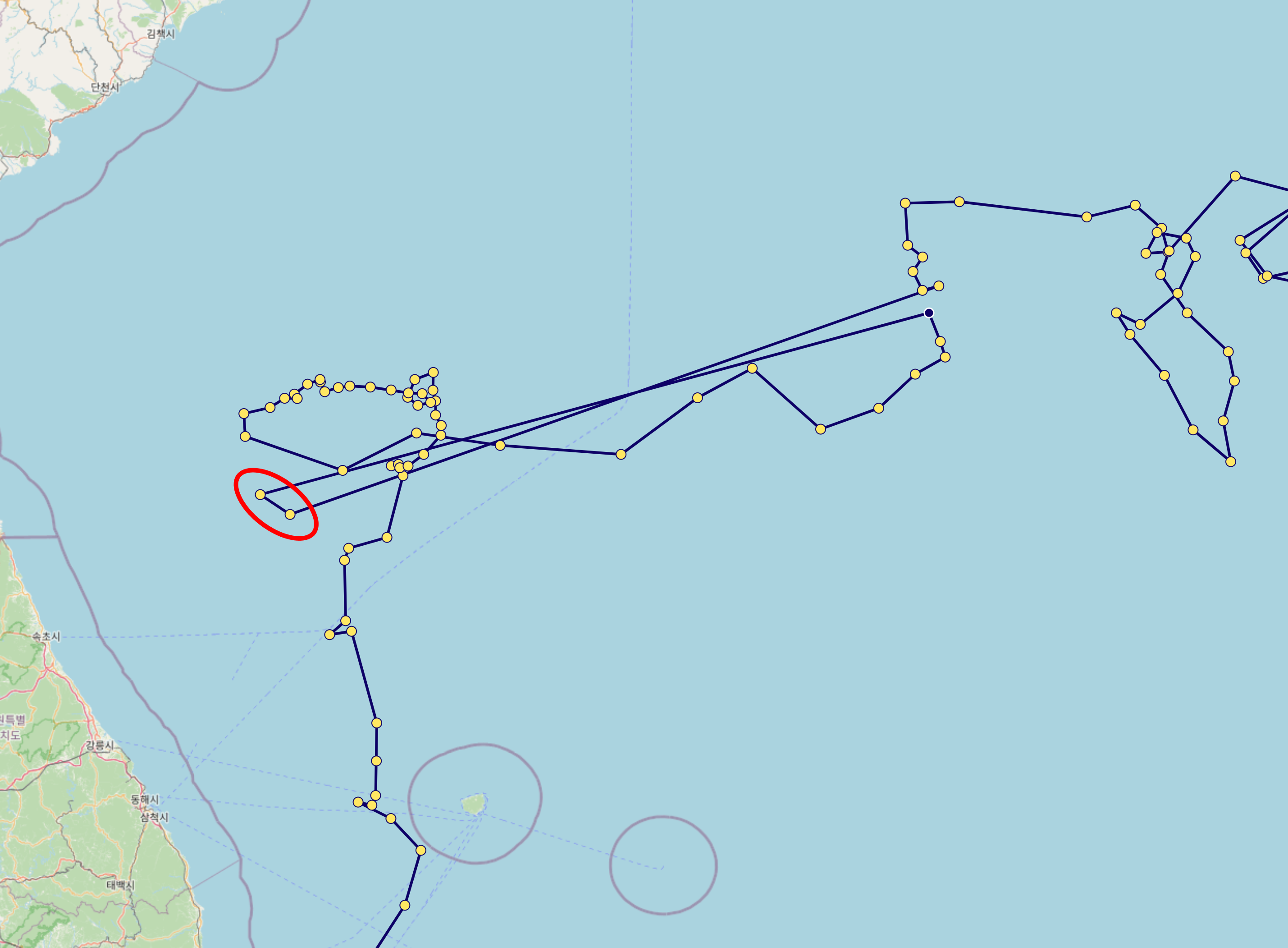
Longitude is normalized to [-180°, 180°] before rounding. Passing position QC does not guarantee that every reported
position is suitable for a particular analysis.
Missing Cells and Numeric Limits
All parameter arrays align with the finite pressure array. A missing cell becomes JSON null; a parameter with no finite
values becomes an empty array. Pressure-only profiles are not published, but a profile can remain available when only a BGC
parameter survives alongside pressure.
After source and QC selection, finite values outside these inclusive ranges become null. They are not clamped, filled, or
retried from another source.
| Parameter | Raw range | ADJUSTED range |
|---|---|---|
| Pressure | 0–2000 dbar | 0–2000 dbar |
| Temperature | -2.5–40.0 °C | -2.5–40.0 °C |
| Practical salinity | 2–41.0 | 2–41.0 |
| Dissolved oxygen | 0–600 µmol/kg | 0–600 µmol/kg |
| Chlorophyll-a | -0.2–100 mg/m³ | -0.1–50 mg/m³ |
| Nitrate | -15–65 µmol/kg | -2–50 µmol/kg |
| BBP700 | -0.000025–0.1 m⁻¹ | -0.000025–0.1 m⁻¹ |
| pH | 7.0–8.8 | 7.3–8.5 |
| Irradiance at 490 nm | -1–3.4 W/m²/nm | -1–3.4 W/m²/nm |
| PAR | -1–4672 µmol quanta/m²/s | -1–4672 µmol quanta/m²/s |
At duplicate pressures, OceanGraph keeps one row deterministically, preferring joint temperature-salinity support and then salinity support. Values from discarded duplicate rows are not merged into the retained row.
Pressure Coverage and Conversion
After the minimum joint-observation count and shallow-coverage checks, profiles with excessive gaps between adjacent joint, acceptable-QC temperature-salinity observations are excluded. The allowed gap increases with pressure because deep observations are typically spaced farther apart. No minimum pressure span or required maximum pressure is imposed.
In-situ temperature is converted to potential temperature, and practical salinity to absolute salinity, with the TEOS-10
Gibbs SeaWater toolbox. A cell-level conversion failure remains null; a failure that removes required joint support can
exclude the profile.
Profile JSON does not interpolate missing cells. Section generation, Akima output, and server-side analyses may interpolate finite values inside a parameter’s observed pressure range, but do not extrapolate beyond it or fill missing profile cycles.
Published values are rounded to the following precision:
| Values | Precision |
|---|---|
| Pressure | 0.01 dbar |
| Temperature, salinity, oxygen, chlorophyll, pH, irradiance | 0.001 |
| Nitrate | 0.01 |
| BBP700 | 0.000001 |
| PAR | 0.1 |
Limitations
Missing Values in Vertical Section Charts
-
Masked Areas Without Original Data
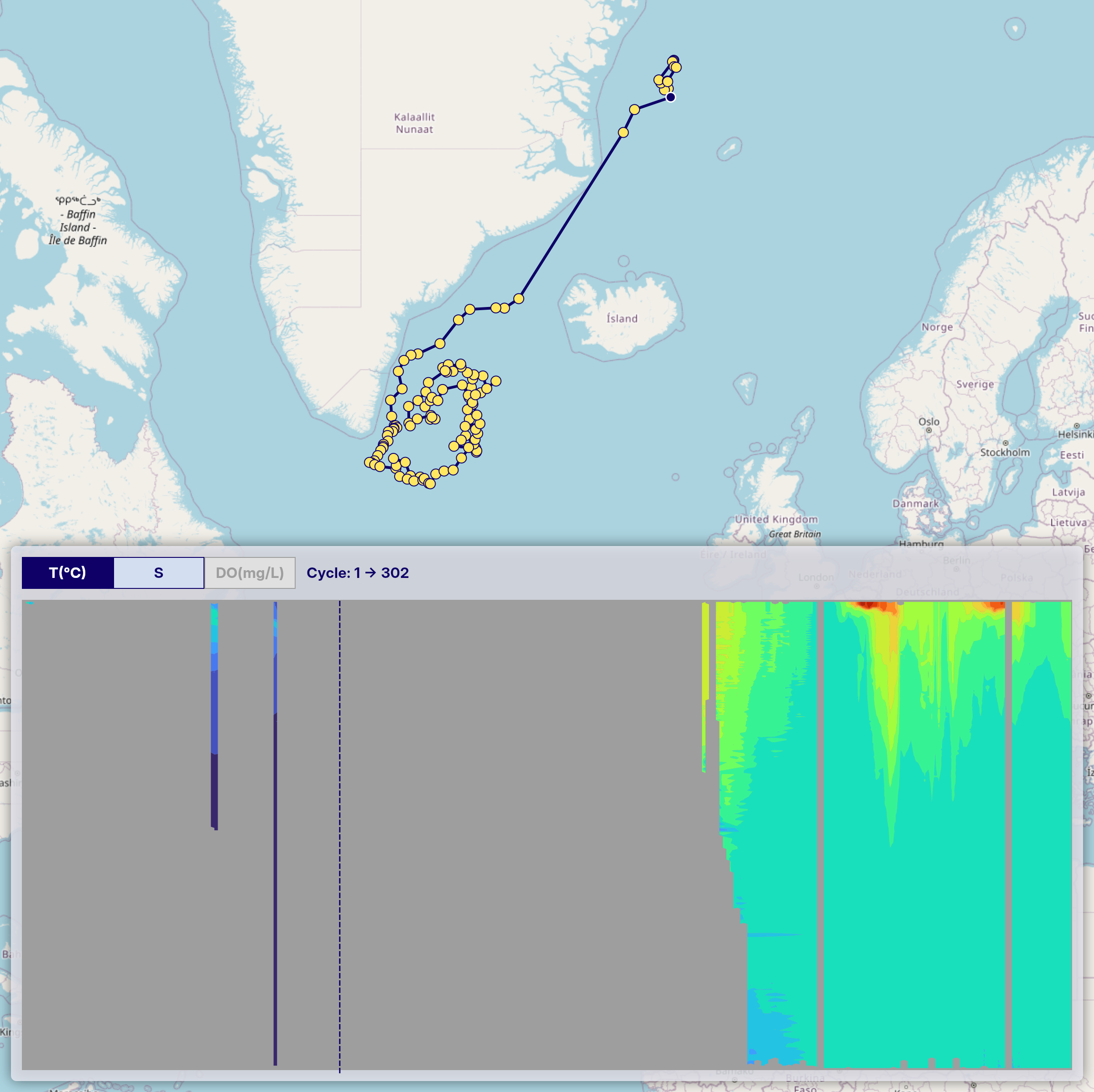
When generating time-series vertical section charts, each profile is interpolated vertically onto a common pressure grid only between finite observations. OceanGraph does not interpolate along the cycle direction. A missing cycle therefore remains a missing column instead of becoming a smooth estimate between distant observations.
In the chart, these masked areas appear as uncolored gaps in the vertical section.
-
Sparse Data Due to Quality Control
After processing, some parameters can have finite values in isolated profiles but no pair of adjacent cycles with enough shared vertical support to form a contour cell. In that case OceanGraph does not publish an SVG for that parameter. The interface distinguishes this “profile data exists, but no drawable section” state from a parameter that has no profile data at all.
A parameter can therefore be available in individual profiles even when the section area reports that no chart can be drawn.
-
BGC Parameter Charts May Have More Missing Areas
Vertical section charts in the OceanGraph interface are also available for BGC parameters (dissolved oxygen, chlorophyll, nitrate, backscattering, pH, and PAR). Because only a subset of Argo floats carry BGC sensors, these variables often contain more
nullcells or isolated cycles than temperature and salinity. Finite BGC measurements are retained independently of missing temperature or salinity cells, but a section still requires adjacent-cycle support to be drawable.PAR observations are typically concentrated in the surface layer (roughly 0–200 dbar), so deeper portions of PAR section charts commonly appear as missing areas.
Note also that of the two irradiance parameters (
DOWN_IRRADIANCE490andDOWNWELLING_PAR), only PAR is displayed as an in-app chart. Downwelling irradiance at 490 nm can make a profile match the “Only profiles with BGC” search filter and is included in downloadable profile data, but it does not have a corresponding in-app visualization.
3D View
The 3D view combines quality-filtered profile values into horizontal surfaces without additional QC. Keep these limits in mind:
- Each variable uses its own valid observations, so BGC values remain available where θ or S is missing. Interpolation stays within each profile’s observed pressure range for that variable; deeper PAR layers commonly remain missing.
- A surface needs valid values at three or more distinct locations that do not lie on one straight line. Repeated profiles at the same location do not add locations.
- Within the area enclosed by valid locations, values are interpolated linearly. Outside that area, the nearest valid value is extended as extrapolation. Both are displayed only at grid points within 250 km of a valid location for that variable and pressure. Distance uses the selected region’s central latitude to scale longitude.
- Areas beyond this limit remain blank, even inside the area enclosed by observations. Blank areas do not mean that the variable is zero or that no water is present.
- The distance limit controls display coverage; it is not a scientific correlation length or an accuracy guarantee. Distant observations can still influence an interpolated value near a valid location.
- Sparse observations and the 0.5° grid can produce coarse contours. Grid spacing and smooth-looking colors do not indicate measurement accuracy.
- Boost contrast expands even small differences across the full palette without changing values or missing areas; colors do not establish scientific significance or identify anomalies. Its scale applies only to the selected layer, so matching colors across layers or after changing depth need not mean matching values.
- Land and seafloor boundaries are ignored.
- Observations from different times are combined without time correction. This exploratory view does not reconstruct a single-time or period-average ocean field. Seasonal and other changes over time can appear as spatial differences, especially in long WMO histories. Check the displayed observation period for every view, including those from geographic searches.
- Horizontal proportions approximate geographic distances, but the pressure direction is exaggerated for readability. The axes do not share one physical distance scale.
Derived Metrics and Mode Water Detection
Derived metrics such as MLD, SOM, and mode water detections are calculated automatically from profiles that pass OceanGraph’s data processing checks. A no-data marker can mean that the source profile was insufficient for the calculation, or that the target feature was not detected under the current criteria.
Mode water detection uses fixed geographic, density, potential vorticity, and minimum-thickness criteria. The default geographic scope is configured to cover broader areas that can include advected mode water signals, but it is still an automatic bounding-box screen and may not cover every scientifically relevant signal. Treat the map data layer and Visual Lab summaries as exploration aids, and inspect the original profile structure when a research-grade classification is required.
Educational Articles
OceanGraph Articles explains the oceanographic concepts and research workflows behind the features documented in this guide. The article site maintains its own current recommendations, categories, and complete article list.
Choose a Language
Feature and data pages in this guide also link directly to the most relevant background article when additional explanation is useful.
Legal Guide
This section contains the legal terms governing your use of OceanGraph. Please review these documents carefully before using the application.
Terms of Service
The Terms of Service cover registration where required, prohibited actions, service changes, warranties and liability, and governing law.
Available in:
Privacy Policy
The Privacy Policy explains how OceanGraph and OceanGraph Articles handle user information.
Available in:
Terms of Service
The Terms of Service are available in the following languages:
Terms of Service
Article 1 (Application and Registration)
These Terms of Service (“Terms”) set forth the conditions for the use of the service “OceanGraph” (“Service”) provided by an individual developer (“we” or “us”) and govern the relationship between us and the users of the Service (“Users”).
By using the Service, Users agree to these Terms. Some features require an account and registration of the requested information.
Article 2 (Prohibited Actions and Account Suspension)
Users must not engage in the following acts:
- Acts that violate laws or public order and morals
- Acts that infringe on the rights of third parties
- Registering false information
- Unauthorized access, excessive loads, or other interference with the operation of the Service
We may suspend a User’s account if the User violates these Terms or if suspension is necessary to maintain the security or operation of the Service.
Article 3 (Changes, Suspension, or Termination of the Service and Data)
We may change, suspend, or terminate the Service for maintenance, system failures, disasters, or other operational or technical reasons.
We do not guarantee the continued availability of the Service or the permanent preservation of user data. We may delete stored user data when the Service ends.
We may, when reasonably necessary to maintain the Service, delete accounts and associated data that have been inactive for an extended period without providing individual advance notice to Users.
Article 4 (Warranties and Liability)
We do not warrant the accuracy, completeness, or fitness for a particular purpose of the Service.
If we are liable in connection with the Service, the scope of that liability will be determined in accordance with applicable law.
Article 5 (Governing Law and Jurisdiction)
These Terms are governed by the laws of Japan. Any dispute relating to these Terms or the Service shall be submitted in the first instance to a Japanese court with jurisdiction under applicable law.
利用規約
第1条(適用および利用登録)
本規約は、個人開発者(以下「当方」といいます)が提供するサービス「OceanGraph」(以下「本サービス」)の利用に関する条件を、本サービスの利用者(以下「ユーザー」)との間で定めるものです。
ユーザーは、本サービスを利用することにより、本規約に同意したものとします。一部の機能を利用するには、アカウント登録および所定の情報の登録が必要です。
第2条(禁止事項および利用停止)
ユーザーは、次の行為をしてはなりません。
- 法令または公序良俗に違反する行為
- 第三者の権利を侵害する行為
- 虚偽の情報を登録する行為
- 不正アクセス、過度な負荷その他本サービスの運営を妨害する行為
当方は、ユーザーが本規約に違反した場合、または本サービスの安全な運営に必要な場合、アカウントの利用を停止できます。
第3条(サービスの変更・停止・終了およびデータ)
当方は、メンテナンス、システム障害、災害その他運営上または技術上必要な場合、本サービスを変更、停止または終了することがあります。
当方は、本サービスの継続的な提供やユーザーデータの永続的な保存を保証しません。本サービスを終了する場合、保存されたユーザーデータを削除することがあります。
当方は、本サービスの維持管理上合理的に必要な場合、長期間利用されていないアカウントおよび関連データを、ユーザーに個別に事前通知することなく削除することがあります。
第4条(保証および責任)
当方は、本サービスの正確性、完全性または特定目的への適合性を保証しません。
当方が本サービスに関して責任を負う場合、その範囲は適用法令に従います。
第5条(準拠法・裁判管轄)
本規約は日本法に準拠します。本規約または本サービスに関する紛争は、法令に従い管轄権を有する日本の裁判所を第一審の管轄裁判所とします。
Privacy Policy
The Privacy Policy is available in the following languages:
Privacy Policy
Last updated: August 3, 2026
This Privacy Policy explains how the individual developer who provides OceanGraph (“we,” “us,” or “our”) handles information in connection with OceanGraph and OceanGraph Articles (collectively, the “Service”).
Article 1 (Information We Collect)
We may collect the following information when providing the Service:
- Account information required for registration and authentication, such as an email address
- Content, contact details, and other information provided through feedback or inquiries
- Usage information such as IP address, usage environment, pages viewed, and interactions with the Service
- Identifiers and settings stored using cookies and similar technologies
OceanGraph does not automatically attach a user ID or email address to feedback content.
Article 2 (Purposes of Use)
We use the information we collect for the following purposes:
- To provide, operate, and maintain the Service
- To verify users and provide authentication features
- To understand usage, improve features and articles, and investigate defects
- To respond to inquiries about the Service and coordinate support
- To prevent and respond to unauthorized use, unauthorized access, and other security issues
Article 3 (Analytics on OceanGraph Articles)
OceanGraph Articles uses Google Analytics 4, provided by Google LLC, only after a user gives consent. We collect information about how articles are viewed and used to understand usage and improve content and navigation. We do not send information entered in the inquiry form to Google Analytics.
OceanGraph Articles stores the user’s analytics choice in the browser. If a user consents to analytics, Google Analytics uses cookies for analytics. Users can change or withdraw consent at any time through “Cookie settings” in the footer of any page. Declining or withdrawing consent does not prevent users from reading articles, switching languages, or following links to OceanGraph.
For details about how Google handles information, see the Google Privacy Policy.
Article 4 (Inquiries on OceanGraph Articles)
We use information submitted through the inquiry form to respond to inquiries and coordinate support. When a user consents to sharing with a partner company, we may share the inquiry and contact details with a suitable partner only to the extent needed to respond.
Article 5 (Service Providers and Disclosure to Third Parties)
We may engage service providers to process information as necessary to provide the Service.
We do not disclose personal information to third parties without the user’s consent, except as permitted by applicable law.
Article 6 (Security)
We take reasonable administrative and technical measures to protect collected information against unauthorized access, loss, alteration, and disclosure.
Article 7 (Contact)
For questions about this Privacy Policy or our handling of user information, please use our contact information.
Article 8 (Changes to This Policy)
We may update this Privacy Policy to reflect changes in law, the Service, or our information practices. If a change is material, we will provide notice through the Service or another appropriate method.
プライバシーポリシー
最終更新日:2026年8月3日
本ポリシーは、個人開発者(以下「当方」といいます)が提供するOceanGraphおよびOceanGraph Articles(以下、総称して「本サービス」といいます)における、ユーザー情報の取扱いについて定めるものです。
第1条(取得する情報)
当方は、本サービスの提供にあたり、次の情報を取得する場合があります。
- アカウント登録・認証に必要なメールアドレス等のアカウント情報
- フィードバックやお問い合わせの際に提供される内容、連絡先その他の情報
- IPアドレス、利用環境、閲覧・操作履歴等の利用情報
- Cookie等に保存される識別子および設定情報
OceanGraphのフィードバック内容に、ユーザーIDやメールアドレスを自動的に付加することはありません。
第2条(利用目的)
取得した情報は、次の目的で利用します。
- 本サービスの提供、運営および保守
- 本人確認および認証機能の提供
- 利用状況の把握、機能や記事の改善および不具合の調査
- 本サービスに関するお問い合わせへの回答および支援の調整
- 不正利用、不正アクセスその他のセキュリティ上の問題の防止および対応
第3条(OceanGraph Articlesのアクセス解析)
OceanGraph Articlesでは、ユーザーが同意した場合に限り、Google LLCが提供するGoogle Analytics 4を使用し、記事の閲覧・利用状況に関する情報を取得します。これらの情報は、記事の利用状況を把握し、内容や導線を改善するために利用します。問い合わせフォームに入力された内容をGoogle Analyticsへ送信することはありません。
OceanGraph Articlesでは、アクセス解析への選択状態をブラウザに保存します。アクセス解析に同意した場合は、Google Analyticsによる解析のためCookieが使用されます。ユーザーは、各ページのフッターにある「アクセス解析の設定」から、いつでも同意を変更または撤回できます。同意しない場合や撤回した場合でも、記事の閲覧、表示言語の切替およびOceanGraphへのリンクは利用できます。
Googleによる情報の取扱いについては、Googleのプライバシーポリシーをご確認ください。
第4条(OceanGraph Articlesのお問い合わせ)
問い合わせフォームから送信された情報は、お問い合わせへの回答および支援の調整に利用します。協力企業への情報共有に同意いただいた場合は、対応に必要な範囲で、お問い合わせ内容および連絡先を対応可能な協力企業へ共有することがあります。
第5条(外部サービスおよび第三者提供)
当方は、本サービスの提供に必要な範囲で、外部事業者へ情報の取扱いを委託することがあります。
当方は、法令上認められる場合を除き、ユーザー本人の同意なく個人情報を第三者へ提供しません。
第6条(安全管理)
当方は、取得した情報の漏えい、滅失、改ざん、不正アクセス等を防止するため、合理的な安全管理措置を講じます。
第7条(お問い合わせ)
本ポリシーまたはユーザー情報の取扱いに関するお問い合わせは、お問い合わせ窓口からご連絡ください。
第8条(プライバシーポリシーの変更)
当方は、法令、サービス内容または情報の取扱いの変更に応じて、本ポリシーを改定することがあります。重要な変更を行う場合は、本サービス上その他の適切な方法でお知らせします。
Contact information
For bug reports, feature requests, and general product feedback, signed-in users with a verified email address can use the OceanGraph feedback form.
For account, security, privacy, or other inquiries, contact us at the address below.